
| 일 | 월 | 화 | 수 | 목 | 금 | 토 |
|---|---|---|---|---|---|---|
| 1 | 2 | 3 | 4 | 5 | 6 | 7 |
| 8 | 9 | 10 | 11 | 12 | 13 | 14 |
| 15 | 16 | 17 | 18 | 19 | 20 | 21 |
| 22 | 23 | 24 | 25 | 26 | 27 | 28 |
| 29 | 30 | 31 |
- teps
- ChatGPT
- 텝스공부
- Julia
- obsidian
- 에러기록
- 수식삽입
- JAX
- 생산성
- Dear abby
- 인공지능
- MATLAB
- Python
- 우분투
- IEEE
- WOX
- 논문작성
- Numerical Analysis
- 옵시디언
- pytorch
- 논문작성법
- 딥러닝
- matplotlib
- 텝스
- 수치해석
- Zotero
- 고체역학
- Linear algebra
- LaTeX
- Statics
- Today
- Total
뛰는 놈 위에 나는 공대생
[딥러닝] Backpropagation을 위한 Automatic differentiation 이론/코딩 본문
[딥러닝] Backpropagation을 위한 Automatic differentiation 이론/코딩
보통의공대생 2022. 7. 9. 16:01이 글에서는 딥러닝에 사용되는 automatic differentiation에 대한 설명을 하고자 한다.
참고한 서적은 Mathematics for machine learning이다.
처음에는 automatic differentiation에 대한 설명을 하고, 이를 딥러닝 백엔드인 PyTorch 결과값을 가지고 이해를 해볼 것이다. 내가 모델에 대해 많이 알고 있지 않아도 요즘은 코드가 잘 되어있어서 쉽게 딥러닝을 테스트해볼 수 있지만 그 구조를 바꾸려면 더 깊은 내용을 알아야 하기 때문에 이 내용을 자세히 살펴볼 필요가 있다.
- 필요한 사전 지식 : Vector, Matrix calculus
- Notation 주의
일반적으로 gradient vector를 column vector로 쓰는 경우가 있고, row vector로 쓰는 경우가 있다. 여기서는 gradient vector를 row vector로 표기한다.
(특이한 것이 기계공학이나 전자전기공학에서는 column vector가 일반적인 것 같은데, 인공지능에서는 gradient를 row vector로 쓴다.)
$\nabla_{\textbf{x}}f = \operatorname{grad}f = \frac{df}{d\textbf{x}}=\begin{bmatrix}
\frac{\partial f(\mathbf{x})}{\partial x_{1}} & \frac{\partial f(\mathbf{x})}{\partial x_{2}} & \cdots & \frac{\partial f(\mathbf{x})}{\partial x_{n}} \\
\end{bmatrix}\in \mathbb{R}^{1\times n}$
1. Automatic differentiation이란?

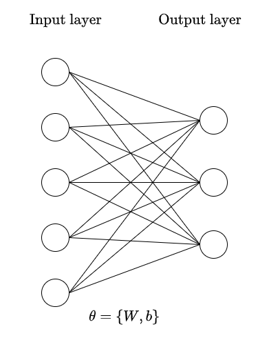
신경망 구조(위 그림)에서는 hidden layer가 하나 밖에 없지만 일반적으로 무수히 많은 layer가 있고 각 layer를 거칠 때마다 weight를 곱하고 bias가 더해진 다음에 설정한 activation function($\sigma$)를 거쳐 hidden layer의 output이 결정된다.
마지막 output layer는 목적에 따라서 다르게 설정할 수 있다.
참고 : 위 그림에서 $h=\sigma(W_{1}x+b_{1})$이 아니라 $h=\sigma(xW_{1}+b_{1})$로 쓴 이유는 PyTorch에서 코딩할 때 사용하는 계산을 그대로 가져온 것이기도 하고, 일반적으로 x의 batch size가 첫 번째 dimension으로 들어가기 때문에 다음과 같이 표기했다.
이 과정에서 우리가 데이터를 가지고 적절히 선정해야하는 것은 weight와 bias들이다. (weight와 bias들을 합쳐서 파라미터parameter라고 부른다. 또한 weight는 $W$, bias는 $b$, 그리고 이 두 개를 모두 합쳐서 $\theta$라고 표기한다.)
이 weight와 bias는 내가 설정한 loss function을 최소화하는 방향으로 움직여야하고, 그래서 gradient descent 방법을 많이 이용한다. 이 방법들에 대해서는 나중에 정리하여 글을 쓸 것이다.
하여튼 이렇게 gradient descent 방법으로 파라미터를 업데이트하려면 loss function($J$)에 대한 파라미터의 미분값을 알아야 한다.
즉, $\displaystyle\frac{dJ}{dW}, \frac{dJ}{db}$에 대해서 알아야하는 것이다. 그런데 층층이 쌓여있는 이전의 weight와 bias에 대한 미분값을 아는 것은 쉽지 않는 일이다. 그래서 나온 것이 automatic differentiation이다.
output layer가 직접적으로 loss function과 관계가 있는 부분이므로 output layer부터 시작하여 순차적으로 각 weight와 bias에 대한 loss function 미분을 구하는 방법이다.
위의 그림을 보았을 때
$\displaystyle \frac{dJ}{d\theta_{2}}=\frac{dJ}{dz}\frac{dz}{d\theta_{2}}$를 구하면
$\theta_{2}=\{W_{2},b_{2}\}$가 변화했을 때 loss function이 어떻게 바뀌는지를 알 수 있다.
또한 $W_{1}$를 업데이트하고 싶다면,
$\displaystyle \frac{dJ}{d\theta_{1}}=\frac{dJ}{dz} \left( \frac{dz}{dh}\frac{dh}{d\theta_{1}}\right)$에 대하여 구하면 된다.
여기서 강조하고 싶은 부분은 $\displaystyle \frac{dJ}{dz}$를 이미 계산을 했다는 사실이다.
지금은 위의 단순한 구조이므로 여기까지만 구하면 $\displaystyle\frac{dJ}{d\theta_{1}},\frac{dJ}{d\theta_{2}}$에 대해서 알기 때문에 gradient descent로 업데이트하면 된다.
Layer 확장
이제 더 많은 layer가 있다고 생각해보면 각 hidden layer의 결과는 $h_{n}$이라고 할 때,
$\displaystyle \frac{dJ}{d\theta_{n}}=\frac{dJ}{dz}\frac{dz}{dh_{N}}\frac{dh_{N}}{dh_{N-1}}\cdots\left(\frac{dh_{n+2}}{dh_{n+1}}\frac{dh_{n+1}}{d\theta_{n}}\right)$
으로 구할 수 있다. 그런데 괄호 친 부분을 제외하고는 이미 $\theta_{k} \; (k\geq n+1)$에 대한 미분을 구할 때 얻은 값들이기 때문에 괄호친 부분만 계산하면 된다.
이런 특성 덕분에 automatic differentiation은 계산량을 줄일 수 있다.
2. 알아두면 유용한 Computing gradients
그런데 automatic differentiation을 할 때 다소 어려운 부분은 바로 벡터와 행렬에 대한 미분이라는 점이다.
위의 있는 식을 하나 가져오자.
$\displaystyle \frac{dJ}{dW_{2}}=\frac{dJ}{dz}\frac{dz}{dW_{2}}$
여기서 $J$는 스칼라, $z$는 벡터이기 때문에 $\frac{dJ}{dz}\in \mathbb{R}^{1\times n}$ 으로 row vector가 나온다.
또한 $\frac{dz}{dW_{2}}$은 벡터를 행렬로 미분한 것이기 때문에 3차원 텐서가 나온다.
이런 경우에는 어떻게 계산해야할까?
mathematics for machine learning 책을 보면 다음과 같은 예제가 있다.
Example $5.12$ (Gradient of Vectors with Respect to Matrices)
Let us consider the following example, where
$$
\boldsymbol{f}=\boldsymbol{A} \boldsymbol{x}, \quad \boldsymbol{f} \in \mathbb{R}^{M}, \quad \boldsymbol{A} \in \mathbb{R}^{M \times N}, \quad \boldsymbol{x} \in \mathbb{R}^{N}
$$
and where we seek the gradient $\mathrm{d} \boldsymbol{f} / \mathrm{d} \boldsymbol{A}$. Let us start again by determining the dimension of the gradient as
$$
\frac{\mathrm{d} \boldsymbol{f}}{\mathrm{d} \boldsymbol{A}} \in \mathbb{R}^{M \times(M \times N)} .
$$
이 문제에서 벡터 $f$가 위의 $z$와 같은 것이다.
실제로 $z=\sigma( hW_{2} +b_{2})$에서 단순하게 생각해서 $\sigma$라는 activation function을 그냥 동일한 결과를 출력하는 함수라고 생각하자. 그러면 위의 문제와 거의 동일하다. 다만 PyTorch에서는 $Ax$가 아니라 $xA$와 같이 표기하므로 dimension에 혼동이 있을 수 있다. 그 부분은 아래에서 PyTorch 예시를 보면서 이해를 하고자 한다.
일단은 위의 예시에 대해서 풀면
$\frac{\mathrm{d} \boldsymbol{f}}{\mathrm{d} \boldsymbol{A}}=\left[\begin{array}{c}\frac{\partial f_{1}}{\partial \boldsymbol{A}} \\ \vdots \\ \frac{\partial f_{M}}{\partial \boldsymbol{A}}\end{array}\right], \quad \frac{\partial f_{i}}{\partial \boldsymbol{A}} \in \mathbb{R}^{1 \times(M \times N)}$
$f$에 대한 $A$ 미분은 각 $f$의 성분을 $A$로 미분한 것을 누적한 것으로 이해할 수 있다.
그런데 앞서 $f=Ax$이므로 이것을 explict하게 작성하면 다음과 같다.
$f_{i}=\sum_{j=1}^{N} A_{i j} x_{j}, \quad i=1, \ldots, M$
그러면 각 $f_{i}$에 대해서 q번째 column은 다음 결과를 얻는다.
$\frac{\partial f_{i}}{\partial A_{i q}}=x_{q}$
즉, $f_{i}$를 미분할 때 i번째 row에만 값을 가지고(나머지는 0이 된다), q번째 column에는 $x_{q}$가 자리잡으므로 사실 상
$\displaystyle\frac{ \mathrm{d} f_{i} }{\mathrm{d} \boldsymbol{A}}=\begin{bmatrix}
0 & \cdots & & & 0 \\
\vdots & & & & \\
\text{(ith row) }x_{1} & x_{2} & \cdots & & x_{N} \\
\vdots & & & & \\
0 & \cdots & & & 0 \\
\end{bmatrix}_{M\times N}$
다음처럼 보이는 것이다.
여기서는 벡터 $x$가 column vector이므로 총체적인 미분은 다음과 같이 표현할 수 있다.
$\frac{\partial f_{i}}{\partial \boldsymbol{A}}=\left[\begin{array}{c}\mathbf{0}^{\top} \\ \vdots \\ \mathbf{0}^{\top} \\ \boldsymbol{x}^{\top} \\ \mathbf{0}^{\top} \\ \vdots \\ \mathbf{0}^{\top}\end{array}\right] \in \mathbb{R}^{1 \times(M \times N)}$
이에 대한 이해를 바탕으로 PyTorch 내에서 gradient를 구해보자.
3. PyTorch 코드 : Automatic differentiation 과정 확인
3.1. Simple case
여기서는
다음과 같은 단순한 신경망 구조에 대해서 gradient를 구한 것을 보여준다.
import torch

x = torch.ones(5)  # input tensor
y = torch.zeros(3)  # expected output
w = torch.randn(5, 3, requires_grad=True)
b = torch.randn(3, requires_grad=True)
z = torch.matmul(x, w)+b
loss = torch.nn.functional.mse_loss(z, y)

print(f"W : {w}")
print(f"b : {b}")
loss.backward()
print(f"gradient w.r.t w : {w.grad}")
print(f"gradient w.r.t b : {b.grad}")
코드를 보면 입력$(x)$은 $[1,1,1,1,1]$로 집어넣고
사용되는 Weight와 bias는 무작위로 뽑았다.
$z = xW + b$로 계산해서 풀었을 때 loss function에 대한 W와 b의 gradient를 구해야 파라미터를 업데이트할 수 있다.
loss function은 $\frac{1}{m}\sum_{i}^{m} (z_{i}-y_{i})^{2}$
output node 수를 m개라고 했을 때 loss는 다음과 같이 mean squared error로 구할 수 있다.
이제 손으로 직접 gradient를 예상해보자.
$\displaystyle\frac{dJ}{dW}$와 $\displaystyle\frac{dJ}{db}$를 알아야 gradient descent 방법을 통해서 update할 수 있다.
$\displaystyle\frac{dJ}{dW}=\frac{dJ}{dz}\frac{dz}{dW}$ 다음과 같이 chain rule를 써서 구해야한다.
여기서 어려운 부분은 z는 벡터이고, W는 행렬이라는 점이다.
위의 예시에서 $z \in \mathbb{R}^{3},\; W\in \mathbb{R}^{5\times 3}$일 때
위의 chain rule 식의 차원은 다음과 같이 정리가 된다.
$\mathbb{R}^{1\times 5 \times 3} = \mathbb{R}^{1\times 3} \cdot \mathbb{R}^{3\times 5\times 3}$
이 문제의 경우에 output node 수가 3개이므로 $m=3$일 때
$\displaystyle\frac{dJ}{dz_{i}}=\frac{1}{3}*2(z_{i}-y_{i})$ 로 구할 수 있다. (위의 loss $\frac{1}{m}\sum_{i}^{m} (z_{i}-y_{i})^{2}$를 미분한 것이다.)
이제 구해야 하는 것은 $\displaystyle\frac{dz}{dW}$를 구해야할 차례이다. 그런데 이 값의 차원은 무려 3*5*3이기 때문에 쉽게 시각화할 수 없다.
그래서 2번에서 다뤘던 벡터에 대한 행렬 미분을 미리 짚고 넘어간 것이다.
$z = xW+b$일 때
$\displaystyle\frac{dz_{i}}{dW} = \begin{bmatrix}
0 & \cdots & \text{(ith column) }x_{1} & \cdots & 0 \\
\vdots & & x_{2} & & \vdots \\
& & \vdots & & \\
& & & & \\
0 & & x_{5} & & 0 \\
\end{bmatrix}_{5\times 3}$
다음과 같은 결과가 나온다. 각각의 $\displaystyle \frac{dz_{i}}{dW}$는 $\frac{dJ}{dz_{i}}$와 곱해진 다음에 그 결과들이 모두 더해진다.
W : tensor([[ 1.7671,  0.2730, -0.4694],
        [-1.0539,  0.5047, -0.2373],
        [-0.9000,  0.2645, -1.4261],
        [-1.5248, -0.2824, -0.0409],
        [-1.0503,  1.4977,  1.6785]], requires_grad=True)
b : tensor([0.5514, 0.6235, 0.6878], requires_grad=True)
gradient w.r.t w : tensor([[-1.4736,  1.9207,  0.1285],
        [-1.4736,  1.9207,  0.1285],
        [-1.4736,  1.9207,  0.1285],
        [-1.4736,  1.9207,  0.1285],
        [-1.4736,  1.9207,  0.1285]])
gradient w.r.t b : tensor([-1.4736,  1.9207,  0.1285])
그러면 우리는
$\begin{bmatrix}
\frac{2}{3}(z_1-y_1) x_{1} & \frac{2}{3}(z_2-y_2) x_{1} & \frac{2}{3}(z_3-y_3) x_{1} \\
\frac{2}{3}(z_1-y_1) x_{2} & \frac{2}{3}(z_2-y_2) x_{2} & \frac{2}{3}(z_3-y_3) x_{2}\\
\frac{2}{3}(z_1-y_1) x_{3} & \frac{2}{3}(z_2-y_2) x_{3} & \frac{2}{3}(z_3-y_3) x_{3} \\
\frac{2}{3}(z_1-y_1) x_{4} & \frac{2}{3}(z_2-y_2) x_{4} & \frac{2}{3}(z_3-y_3) x_{4} \\
\frac{2}{3}(z_1-y_1) x_{5} & \frac{2}{3}(z_2-y_2) x_{5} & \frac{2}{3}(z_3-y_3) x_{5} \\
\end{bmatrix}_{1\times 5\times 3}$
라는 결과를 얻는다. PyTorch는 $(1,5,3)$ 사이즈는 squeeze를 통해 차원 하나를 줄이는 것으로 보인다.
위 결과를 보면 W에 대한 gradient가 아래처럼 나오는데
gradient w.r.t w =
[[-1.4736,  1.9207,  0.1285],
 [-1.4736,  1.9207,  0.1285],
 [-1.4736,  1.9207,  0.1285],
 [-1.4736,  1.9207,  0.1285],
 [-1.4736,  1.9207,  0.1285]]
x,y,z 벡터를 확인하면
print(f"x : {x}")
print(f"z : {z}")
print(f"y : {y}")

x : tensor([1., 1., 1., 1., 1.])
z : tensor([-2.2104,  2.8811,  0.1927], grad_fn=<AddBackward0>)
y : tensor([0., 0., 0.])
다음과 같으므로
이는 $\frac{2}{3}(z_{1}-y_{1})=\frac{2}{3}(-2.2104-0)=-1.4736$을 계산한 결과 등 모두 일치하는 것을 확인할 수 있다.
마찬가지로 bias에 대해서 생각하면
$\displaystyle \frac{dJ}{db}=\frac{dJ}{dz}\frac{dz}{db}$ 다음을 구해야한다.
$\displaystyle\frac{dJ}{dz}$는 이미 알고 있고 $\displaystyle\frac{dz}{db}$는 bias는 벡터이고 $z$도 벡터이기 때문에 행렬이 나온다.
$z=xW+b$ 를 고려하면
$\displaystyle\frac{dz}{db}=\begin{bmatrix}
1 & 0 & 0 \\
0 & 1 & 0 \\
0 & 0 & 1 \\
\end{bmatrix}$이다.
따라서 계산하면 위의 bias 미분결과인
gradient w.r.t b : tensor([-1.4736, 1.9207, 0.1285])와 일치한다.
3.2. Advanced case (보충할 예정)
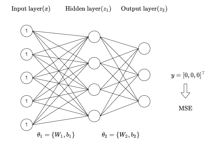
이번에는 hidden layer를 추가한다. 좀 더 복잡해지는데 그래도 activation function이 추가되지 않아서 계산하기 쉬운 편이다. activation function이 추가된다면 chain rule을 적용해서
$z = \sigma(hW+b)$
$\displaystyle\frac{dJ}{dW}=\frac{dJ}{dz}\frac{dz}{dW}=\frac{dJ}{dz} \left(\sigma'(hW+b)\right)\cdot \frac{hW+b}{dW}$
다음처럼 구할 수 있다. $\sigma'$는 activation function을 미분한 결과이다.
input layer는 동일한 5개 node에 모두 1이 들어가고, hidden layer는 node 4개, 마지막 output layer는 node 3개이다.
x = torch.ones(5)  # input tensor
y = torch.zeros(3)  # expected output
w1 = torch.randn(5, 4, requires_grad=True)
b1 = torch.randn(4, requires_grad=True)
z1 = torch.matmul(x, w1)+b1
w2 = torch.randn(4, 3, requires_grad=True)
b2 = torch.randn(3, requires_grad=True)
z2 = torch.matmul(z1, w2)+b2
loss = torch.nn.functional.mse_loss(z2, y)
다음과 같이 x,y는 고정해놓고 중간에 곱해지는 layer들의 값들을 랜덤으로 추출한다.
마지막에 loss는 mse로 들어간다. 그렇게 했을 때 각 weight와 bias는 다음과 같다.
W1 : tensor([[ 1.0428, -0.3946,  0.7416,  0.1335],
        [-1.4995,  1.3843,  0.4623, -0.2594],
        [-0.9014,  0.3262,  0.5743,  1.4366],
        [-0.7088, -0.1805,  0.0337,  0.6872],
        [-2.3582, -2.3633,  1.0293,  0.4191]], requires_grad=True)
b1 : tensor([-1.5663,  1.6879,  0.7603,  0.1443], requires_grad=True)
W2 : tensor([[ 0.3342,  0.1324,  0.4231],
        [-0.2909,  0.4188, -0.6239],
        [ 1.7661,  0.1598,  2.3778],
        [-0.6380, -0.2140, -0.1464]], requires_grad=True)
b2 : tensor([-0.6040,  1.3098,  0.6254], requires_grad=True)
또한 backward를 수행했을 때,
gradient w.r.t w1 : tensor([[ 2.1977, -2.6716, 11.9156, -1.5348],
        [ 2.1977, -2.6716, 11.9156, -1.5348],
        [ 2.1977, -2.6716, 11.9156, -1.5348],
        [ 2.1977, -2.6716, 11.9156, -1.5348],
        [ 2.1977, -2.6716, 11.9156, -1.5348]])
gradient w.r.t b1 : tensor([ 2.1977, -2.6716, 11.9156, -1.5348])
gradient w.r.t w2 : tensor([[ -7.9341,  -2.9428, -23.9331],
        [  0.6091,   0.2259,   1.8373],
        [  4.7694,   1.7690,  14.3867],
        [  3.3918,   1.2580,  10.2313]])
gradient w.r.t b2 : tensor([1.3243, 0.4912, 3.9947])
각 파라미터들의 gradient는 다음과 같다.
각 layer의 값들은 다음과 같다.
x : tensor([1., 1., 1., 1., 1.])
z1 : tensor([-5.9913,  0.4599,  3.6015,  2.5612], grad_fn=<AddBackward0>)
z2 : tensor([1.9864, 0.7368, 5.9920], grad_fn=<AddBackward0>)
y : tensor([0., 0., 0.])
파라미터를 랜덤으로 뽑는 과정에서 숫자들이 조금 귀찮게 나온 것은 사실이지만 차근차근 gradient를 구하도록 한다.
PyTorch 내부에서는 좀 더 효율적으로 계산이 될 텐데
내가 직접 시도를 할 때는 3차원 텐서의 계산이 어떤 방식으로 동작되는지 알기 못해서 코드를 바꿔가면서 시도해보았다.
첫 번째로 구할 것은
$\displaystyle\frac{dJ}{dW_{2}}=\frac{dJ}{dz_{2}}\frac{dz_{2}}{dW_{2}}$이다.
$\displaystyle\frac{dJ}{dz_{2}}$는 mse를 $z_{2}$에 대해서 미분한 것이므로 $\frac{2}{3}(z_{2}-y)$로 구할 수 있다.
$\frac{2}{3}$은 제곱에서 미분할 때 나온 2와 총 output layer의 node 3개를 나눠준 것이다.
또한 $\frac{dz_{2}}{dW_{2}}\in \mathbb{R}^{3\times 4 \times 3}$는 벡터를 행렬로 미분한 것이기 때문에 복잡하지만, 위의 2번 항목에서 벡터를 행렬로 미분한 결과를 참고하도록 하자.
$z_{2}=z_{1}W_{2}+b_{2}$이므로
나머지가 다 0이고
$z_{1}\in\mathbb{R}^{4\times 1}$이 된다.
dz_dw2 = torch.zeros(z2.size(dim=0),w2.size(dim=0),w2.size(dim=1))
dJ_dz = 2/3 * (z2 - y)

for i in range(z2.size(dim=0)):
    dz_dw2[i,:,i] = z1

dJ_dw2 = torch.matmul(dz_dw2,dJ_dz)
print(f"calculate the gradient of w2 : \n{dJ_dw2}")
print(f"dz_dw2 size : {dz_dw2.size()}")
print(f"dJ_dz size : {dJ_dz.size()}")
print(f"dJ_dw2 size : {dJ_dw2.size()}")
calculate the gradient of w2 :
tensor([[ -7.9341, 0.6091, 4.7694, 3.3918],
[ -2.9428, 0.2259, 1.7690, 1.2580],
[-23.9331, 1.8373, 14.3867, 10.2313]],
grad_fn=<UnsafeViewBackward0>)
dz_dw2 size : torch.Size([3, 4, 3])
dJ_dz size : torch.Size([3])
dJ_dw2 size : torch.Size([3, 4])다음과 같이 계산하면,
직접 계산한 W2에 대한 gradient는
위의 backward로 구한 결과(아래)와 같다.
gradient w.r.t w2 : tensor([[ -7.9341,  -2.9428, -23.9331],
        [  0.6091,   0.2259,   1.8373],
        [  4.7694,   1.7690,  14.3867],
        [  3.3918,   1.2580,  10.2313]])
결과에서 transpose된 것 빼고는 동일하다.
그러면 (4,3)으로 나오게 할 수는 없을까? 이 고민은 matmul 에 대한 이해를 동반해야한다.(다음글과 함께 보면 좋다.)
위의 matmul이 이뤄지는 원리가 까다롭다.
위 코드에서는 곱셈의 순서가 $\frac{dz_{2}}{dW_{2}} * \frac{dJ}{dz_{2}}$인데
이는 3차원 텐서와 1차원의 곱에서
(3,4,3) * (3,1) = (3,4)로 나온 것이다.
$\frac{dJ}{dz_{2}}*\frac{dz_{2}}{dW_{2}}$로 계산하고 싶었는데 그렇게 하려면
dz_dw2 = torch.zeros(w2.size(dim=0),w2.size(dim=1),z2.size(dim=0))
dJ_dz = 2/3 * (z2 - y)
for i in range(z2.size(dim=0)):
    dz_dw2[:,i,i] = z1

dJ_dw2 = torch.matmul(dJ_dz,dz_dw2)
print(f"calculate the gradient of w2 : {dJ_dw2}")
print(f"dz_dw2 size : {dz_dw2.size()}")
print(f"dJ_dz size : {dJ_dz.size()}")
print(f"dJ_dw2 size : {dJ_dw2.size()}")
calculate the gradient of w2 : tensor([[ -7.9341, -2.9428, -23.9331],
[ 0.6091, 0.2259, 1.8373],
[ 4.7694, 1.7690, 14.3867],
[ 3.3918, 1.2580, 10.2313]], grad_fn=<ReshapeAliasBackward0>)
dz_dw2 size : torch.Size([4, 3, 3])
dJ_dz size : torch.Size([3])
dJ_dw2 size : torch.Size([4, 3])다음과 같이 (3) * (4,3,3) = (4,3)이 된다.
그 이유는 matmul에서 3차원 텐서가 뒤에 곱해질 때, 맨 앞의 dimension 4는 batch size처럼 되어서 계산을 안하고, 3*(3,3) = 3으로 계산을 하기 때문이다.
덕분에 위의 결과는 backward로 구한 결과와 동일하게 된다.
위의 $\displaystyle\frac{dz_{2}}{dW_{2}}$를 출력하면
print(dz_dw2[:,:,0])
print(dz_dw2[:,:,1])
print(dz_dw2[:,:,2])
tensor([[-5.9913, 0.0000, 0.0000],
[ 0.4599, 0.0000, 0.0000],
[ 3.6015, 0.0000, 0.0000],
[ 2.5612, 0.0000, 0.0000]], grad_fn=<SelectBackward0>)
tensor([[ 0.0000, -5.9913, 0.0000],
[ 0.0000, 0.4599, 0.0000],
[ 0.0000, 3.6015, 0.0000],
[ 0.0000, 2.5612, 0.0000]], grad_fn=<SelectBackward0>)
tensor([[ 0.0000, 0.0000, -5.9913],
[ 0.0000, 0.0000, 0.4599],
[ 0.0000, 0.0000, 3.6015],
[ 0.0000, 0.0000, 2.5612]], grad_fn=<SelectBackward0>)
$z_{1}$ 벡터가 각 column에 들어가있다. 위의 2번에서는
$\displaystyle\frac{ \mathrm{d} f_{i} }{\mathrm{d} \boldsymbol{A}}=\begin{bmatrix}
0 & \cdots & & & 0 \\
\vdots & & & & \\
\text{(ith row) }x_{1} & x_{2} & \cdots & & x_{N} \\
\vdots & & & & \\
0 & \cdots & & & 0 \\
\end{bmatrix}_{M\times N}$
으로 row에 x가 자리잡았지만,
PyTorch에서는 계산이 $xW+b$으로 row vector가 default이기 때문에
전체적으로 transpose로 생각해야한다는 것을 알 수 있었다.
즉, (dim_1, dim_2, dim_3)이 있을 때
$\displaystyle\frac{dz_{2}}{dW_{2}}\text{ where} z_{2}\in\mathbb{R}^{3}, W_{2}\in{4\times 3}$일 때
$\displaystyle\frac{dz_{2}}{dW_{2}}$는 $(4\times3) * 3$ 으로 구성을 해야한다. $(4\times 3)$은 $W_{2}$에 의한 것이고 마지막 3은 $z_{2}$에 의한 것이다.
또한 그 다음 스텝으로 가서
$\displaystyle\frac{dJ}{dW_{1}}=\frac{dJ}{dz_{2}}\frac{dz_{2}}{d_{z_{1}}}\frac{dz_{1}}{dW_{1}}$을 구해야한다.
$dJ/dz_{2}\in\mathbb{R}^{3}=\frac{2}{3}(z_{2}-y)$는 앞서 구했고,
$z_{2}=z_{1}W_{2}+b_{2}$ 관계이기 때문에 $\frac{dz_{2}}{dz_{1}}$은 $W_{2}\in \mathbb{R}^{4\times 3}$의 transpose가 된다. gradient의 notation에 따라 달라질 수는 있지만 그렇다,
그리고 $z_{1}=xW_{1}+b_{1}$이므로 $\frac{dz_{1}}{dW_{1}}\in \mathbb{R}^{5\times 4\times 4}$는
tensor([[1., 0., 0., 0.],
        [1., 0., 0., 0.],
        [1., 0., 0., 0.],
        [1., 0., 0., 0.],
        [1., 0., 0., 0.]])
tensor([[0., 1., 0., 0.],
        [0., 1., 0., 0.],
        [0., 1., 0., 0.],
        [0., 1., 0., 0.],
        [0., 1., 0., 0.]]) ...
등으로 구성된 3차원 텐서이다. (각 column이 모두 1인 이유는 x의 모든 원소가 1이기 때문이다.)
W2 = torch.tensor([[ 0.3342,  0.1324,  0.4231],
        [-0.2909,  0.4188, -0.6239],
        [ 1.7661,  0.1598,  2.3778],
        [-0.6380, -0.2140, -0.1464]])
x = torch.ones(5)
z2 = torch.tensor([1.9864, 0.7368, 5.9920])

dz_dw1 = torch.zeros((5,4,4))
for i in range(4):
    dz_dw1[:,i,i] = x

init = torch.matmul(2/3*z2, W2.T)
gradient = torch.matmul(init,dz_dw1)
다음을 통해 계산한 $\displaystyle\frac{dJ}{dW_{1}}$(위 코드의 gradient)은
tensor([[ 2.1977, -2.6718, 11.9158, -1.5348],
        [ 2.1977, -2.6718, 11.9158, -1.5348],
        [ 2.1977, -2.6718, 11.9158, -1.5348],
        [ 2.1977, -2.6718, 11.9158, -1.5348],
        [ 2.1977, -2.6718, 11.9158, -1.5348]])
다음과 같고 이는 backward로 구한 값과 일치한다.
gradient w.r.t w1 : tensor([[ 2.1977, -2.6716, 11.9156, -1.5348],
        [ 2.1977, -2.6716, 11.9156, -1.5348],
        [ 2.1977, -2.6716, 11.9156, -1.5348],
        [ 2.1977, -2.6716, 11.9156, -1.5348],
[ 2.1977, -2.6716, 11.9156, -1.5348]])'연구 Research > 인공지능 Artificial Intelligent' 카테고리의 다른 글
| [PyTorch] retain_graph = True라고 했음에도 backward 문제가 발생하는 경우 (0) | 2023.01.05 |
|---|---|
| [PyTorch] 모델 저장/불러오기 및 모델 수정하기 (0) | 2023.01.04 |
| [인공지능] CUDA & cuDNN 설치하는 방법 (0) | 2021.08.30 |
| [머신러닝] Boosting method (0) | 2021.05.26 |
| [머신러닝] Logistic Regression (0) | 2021.05.25 |

