이번에는 explicit euler 방법이 아닌 implicit euler 방법을 사용하고자 합니다.
# Notation 참고
: 는 시간에서의 위치(Timesteps), 는 공간에서의 위치를 의미합니다.
model problem인 을 implicit euler 방법으로 풀어보겠습니다.
: implicit euler이므로 현재 y,t값이 아닌 미래의 값(n+1)을 사용합니다.
1) Accuracy
두 개를 비교하면 그 errors는 second order in a time step입니다. globally first order accuracy.
2) Stability
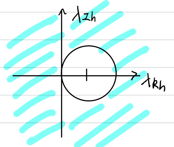
앞서 explicit euler에서처럼 amplication factor가 1보다 작아야 stable solution을 얻을 수 있습니다.
위 조건에 맞는 영역은

일 때 implicit euler 방법을 쓰면 항상 solution이 stable하므로, implicit euler는 Absolutely stable(A-stable)입니다.
인 영역은 원래 unstable system이므로 고려하지 않지만, 만약 unstable한 문제를 풀 때도 위 그림처럼 stable한 solution이 나온다면 문제가 될 수도 있습니다.
3) Phase error & amplitude error
이전 explicit euler때처럼 일 때 phase error와 amplitude error를 알아보겠습니다.
stability diagram을 통해 알 수 있듯이 pure imaginary에서 implicit euler는 decaying합니다.
또한 phase error =
exact값은 이므로
4) Implicit euler의 특징
larger memory space is needed
flexbility in time-step
nonlinear equation에 대해서 iteration이 필요함
5) Explicit euler와 비교
model problem에 대해서
둘은 same order of accuracy를 가졌지만 부호가 다릅니다.
implicit euler는 explicit euler와 다르게 A-stable이지만 실제 사용하기에는 accuracy order가 낮다는 단점을 가지고 있습니다.
'수치해석 Numerical Analysis' 카테고리의 다른 글
| [수치해석] Numerical solution of ODE (5) Predictor-Corrector Method (0) | 2021.09.26 |
|---|---|
| [수치해석] Numerical solution of ODE (4) Trapezoidal method (Crank-Nicolson) (0) | 2021.09.24 |
| [수치해석] Numerical solution of ODE (2) Explicit Euler (0) | 2021.04.27 |
| [수치해석] Numerical solution of ODE (1) introduction (0) | 2021.04.07 |
| [수치해석] Numerical integration (3) - Gauss quadrature (0) | 2021.04.04 |