[수치해석] Numerical integration (3) - Gauss quadrature

이번에는 numerical integration의 마지막, Gauss quadrature에 대해서 알아보겠습니다.

 

1. Definition of Gauss quadrature

 

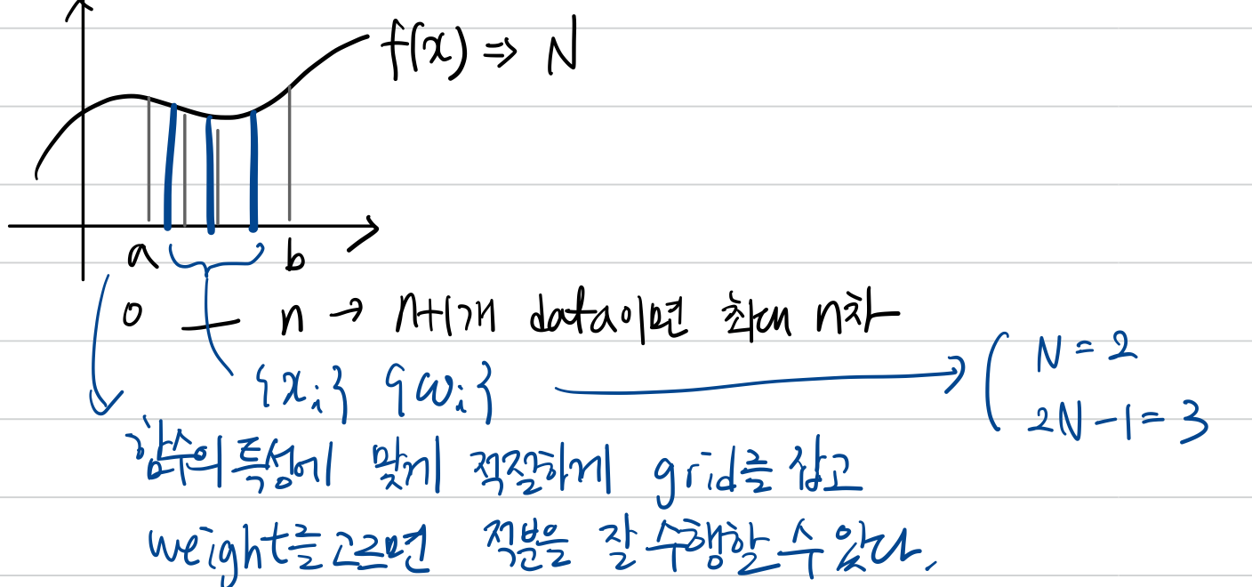
Gauss quadrature는 특정 weight($w_{i}$)와 함수값 ($f(x_{i})$)의 곱을 discrete하게 더했을 때 그 구간의 definite integral과 거의 approximate하게 만드는 방법입니다.

식으로 표현하면 다음과 같습니다.

$\int_{a}^{b} f(x) dx \approx \sum_{i=0}^{n}f(x_{i})\cdot w_{i}\cdots\cdots (*)$

 

이 때, $h\text{ (interval between the points)}, \{w_{i}\}, \{x_{i}\}$는 균일한 값을 가질 수도 있고, 아닐 수도 있습니다.

uniform하지 않은 간격과 weight를 가질 수 있다는 뜻.

 

Gauss quadrature는 여러가지 variation을 가지고 있습니다. Gauss quadrature를 어떤 integration technique의 한 class라고 볼 수도 있습니다.

Gauss quadrature 방법에는

$\text{Gauss-Legendre, Gauss-Chebyshev, Gauss-Hermite, Gauss-Laguere}$ 등이 있습니다.

 

cf) 위의 방법의 발음은 각각 가우스-르장드르, 가우스-체비쇼프, 가우스-에르미트, 가우스-라게르 라고 합니다.

 

Gauss quadrature의 정의 :

$\text{Let }q(x)\text{ is a polynomial of degree N such that }$

$\int_{a}^{b}q(x)\rho(x)x^{k}dx=0\text{ where k is any integer in }[0,N-1]\text{ and }\rho (x)\text{ is a weighting function.}$

$\text{Let }\{x_{i}\} \text{ be the N roots of }q(x)\text{ construct the integration formula (*),}$

$\text{we guarantee that for some set of }\{w_{i}\}\text{ the (*) is exact if }f(x)\text{ is a polynomial of degree <2N-1>}$

 

 

 

2. Gauss quadrature

 

$\int_{a}^{b}q(x)\rho(x) x^{k}dx=0$

여기서 $q(x)$는 변수입니다.

k는 [0,N-1]일 때 위 식을 만족하는 $q(x)$를 구하고 $q(x)$의 roots($\{x_{i}\}$)를 구한 다음에

 

$\int_{a}^{b}f(x)dx \triangleq \sum_{i=0}^{n}w_{i}f(x_{i})$

(f(x)의 order가 2N보다 작다고 가정)

위 식에 대입해서 이를 만족하는 $w_{i}$를 구하면 exact하게 적분값을 구할 수 있습니다.

 

 

example : 3-point Gauss Legendre quadrature

1) 3 grid points (i=0,1,2) 사용 (N=3)

2) $\rho(x)=1$ weighting function은 1이라고 가정

3) integrate on [-1,1] : [-1,1] 적분으로 만들기 위해 variable x를 변형함

$\int_{a}^{b}f(x)dx=\frac{(b-a)}{2}\int_{-1}^{1}f(u)du \text{, where }x=\frac{1}{2}(b+a)+\frac{1}{2}(b-a)u$

 

 

Step1) Find $q(x)$

 

N=3이므로 $q(x)$는 3차 polynomial입니다.

$q(x)=c_{0}+c_{1}x+c_{2}x^{2}+c_{3}x^{3}$

 

위의 정의에서 $k \text{ for }x^{k}$는 $[0,2]$ 안에서 결정되어야 합니다.

 

$\left\{\begin{matrix} k=0:&\int_{-1}^{1}(c_{0}+c_{1}x+c_{2}x^{2}+c_{3}x^{3})\cdot 1\cdot x^{0}dx=0&\cdots (1)\\  k=1:&\int_{-1}^{1}(c_{0}+c_{1}x+c_{2}x^{2}+c_{3}x^{3})\cdot 1\cdot x^{1}dx=0&\cdots (2) \\  k=2:&\int_{-1}^{1}(c_{0}+c_{1}x+c_{2}x^{2}+c_{3}x^{3})\cdot 1\cdot x^{2}dx=0&\cdots (3)   \end{matrix}\right.$

 

$2c_{0}+\frac{2}{3}c_{2}=0$

$\frac{2}{3}c_{1}+\frac{2}{5}c_{3}=0$

$\frac{2}{3}c_{0}+\frac{2}{5}c_{2}=0$

 

이 세 개의 식을 연립하여 $c_{0},c_{1},c_{2},c_{3}$를 구하고 싶지만 식은 3개인데 문자가 4개이므로 해는 무수히 많습니다.

따라서 위 연립방정식을 풀었을 때 $q(x)=-ax+\frac{5}{3}ax^{3}$ 다음과 같이 나옵니다. $a$는 0이 아닌 임의의 숫자가 들어갈 수 있지만, $a=\frac{3}{2}$일 때 $q(x)=-\frac{3}{2}x+\frac{5}{2}x^{3}$

 

 

Step 2) Find roots of $q(x)$

 

$q(x)$의 roots를 구하기 위해서 $q(x)=0$을 풉니다.

 

$q(x)$의 roots는 $\{x_{i}\}=\pm \sqrt{\frac{5}{3}},0$

 

 

Step 3) Find $w_{i}$

 

$\int_{-1}^{1}f(x)dx=\sum_{i=0}w_{i}f(x_{i})=w_{0}f(x_{0})+w_{1}f(x_{1})+w_{2}f(x_{2})=w_{0}f\left(-\sqrt{\frac{3}{5}}\right)+w_{1}f(0)+w_{2}f\left(\sqrt{\frac{3}{5}}\right)$

 

 

이 때 $f(x)={1,x,x^{2},x^{2},x^{3},x^{4},x^{5}}$까지 $2N-1=5$차 order까지 표현할 수 있습니다.

각각의 $f(x)$에서 적분값과 weight, roots의 함수값의 summation이 동일하도록 만듭니다.

 

$\int_{-1}^{1}1 dx=2=w_{0}f\left(-\sqrt{\frac{3}{5}}\right)+w_{1}f(0)+w_{2}f\left(\sqrt{\frac{3}{5}}\right)=w_{0}+w_{1}+w_{2} \quad (\because f(x)=1)$

 

$\int_{-1}^{1}x dx=0=w_{0}\cdot\left(-\sqrt{\frac{3}{5}}\right)+w_{1}\cdot 0+w_{2}\cdot\left(\sqrt{\frac{3}{5}}\right)$

 

$\int_{-1}^{1}x^{2} dx=\frac{2}{3}=w_{0}\cdot\left(-\sqrt{\frac{3}{5}}\right)^{2}+w_{1}\cdot 0^{2}+w_{2}\cdot\left(\sqrt{\frac{3}{5}}\right)^{2}$

 

이렇게 3개의 식으로 $w_{0},w_{1},w_{2}$을 구하면 $w_{0}=\frac{5}{9},w_{1}=\frac{8}{9},w_{2}=\frac{5}{9}$가 나옵니다.

 

이 weight를 나머지 $f(x)=x^{3},x^{4},x^{5}$에 넣으면

$x^{3},x^{5}$는 기함수이기 때문에 $[-1,1]$ 적분에서 0으로 사라지고(좌변) weight를 집어넣을 때도 우변이 0으로 되므로 성립합니다.

 

$f(x)=x^{4}$일 때

$\int_{-1}^{1}x^{4} dx=\frac{2}{5}=\frac{5}{9}\cdot\left(-\sqrt{\frac{3}{5}}\right)^{4}+\frac{8}{9}\cdot 0^{4}+\frac{5}{9}\cdot\left(\sqrt{\frac{3}{5}}\right)^{4}$

 

$f(x)=x^{6}$일 때는 $\int_{-1}^{1}x^{6} dx=\frac{2}{7}\neq2\cdot \frac{5}{9}\cdot\frac{27}{125}$

성립하지 않습니다.

 

따라서 3개의 points가 주어졌을 때 $f(x)$가 5차 polynomial일 때까지 exact하게 적분을 수행할 수 있습니다.

 

 

또한 위에서 구한 $q(x)=-\frac{3}{2}x+\frac{5}{2}x^{3}$은 Legendre polynomial of degree 3입니다.

 

$\text{Legendre Polynomial }P_{n}(x)=\frac{1}{n!2^{n}}\frac{d^{n}}{dx^{n}}(x^{2}-1)^{n} (n=0,1,2,\ldots)$

 

또한 weight를 구하는 공식도 이미 나와있습니다.

 

$w_{i}=\frac{2}{(1-x_{i}^{2})(P_{N}^{'}(x_{i}))}$

 

---

위의 방법은 Gauss-Legendre method이었고 그 외에 다른 방법이 있다는 것을 이미 언급했습니다.

 

만약 적분이

$\int_{0}^{\infty}e^{-x}f(x)dx$라면

Gauss-Laguere를 쓰는 게 더 좋습니다.

 

$\int_{-\infty}^{\infty}e^{-x^{2}}f(x)dx \text{ : Gauss-Hermite}$

$\int_{-1}^{1}\frac{f(x)}{\sqrt{1-x^{2}}}dx \text{ : Gauss-Chebyshev}$

 

내가 함수의 형태를 알고 있다면 그에 맞춰서 위 방법 중에 택하여, table에서 weight 및 roots값을 찾을 수 있다고 합니다.