Laplace transform과 Z transform은 비슷한 성격이 많아서, 나중에 비교를 하는 글도 따로 마련할 예정입니다.
여기서 다루는 Laplace transform은 엄밀하게 따져서 Unilateral Laplace transform입니다.
(Bilateral) Laplace transform은 정의 상 $\int_{-\infty}^{\infty} f(t) e^{-st} dt $ 이지만, 물리적인 현상에서 $ f(t)=0, t<0 $라고 보기 때문에 Unilateral Laplace transform의 정의인 $\int_{0}^{\infty} f(t) e^{-st} dt $을 사용합니다.
따라서 아래에서 제가 Laplace transform이라고 말할 때는 Unilateral Laplace transform을 의미한다는 것을 염두해주시기 바랍니다. (왜냐하면 properties에서 일반적인 laplace transform과 다를 수 있기 때문입니다.)
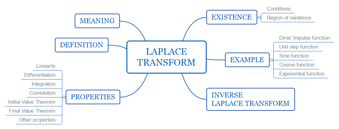
1. Meaning
Laplace transform은 Ordinary Differential Equation을 푸는데 유용한 방법입니다.
Linear Differential Equation을 Laplace transform을 통해 대수적인 방정식 형태로 바꾸고, 그 방정식에서 해를 구한 다음 Inverse Laplace transform을 이용해 해를 구합니다.
저는 laplace transform이 time domain에서 s-domain으로 전환한 다음, s-domain에서 풀고 이 결과를 time domain으로 바꿔서 문제를 풀 때 domain을 바꿔주는 방식(법칙, 함수 등)이라고 기억합니다. 마치 선형대수에서 transformation matrix을 이용해서 푸는 것처럼 말이죠.
2. Definition
$ \text{Continuous function} f : \Re_{+} \rightarrow \Re $
$\text{Laplace transform } F(s)= \mathcal{L} \{f(t)\} \triangleq \int_{0}^{\infty} f(t) e^{-st} dt, s\in\mathbb{C}$
$\text{Inverse Laplace transform } f(t)=\frac{1}{2\pi j}\int_{\sigma+j\infty}^{\sigma-j\infty} F(s) e^{st} ds$
inverse Laplace transform공식은 fourier transform에서 synthesis equation을 통해서 구할 수 있습니다.
# fourier transform을 이용해 inverse Laplace transform을 구하는 과정
$\text{Fourier transform } x(t) = \frac{1}{2\pi} \int_{-\infty}^{\infty} X(j\omega) e^{j \omega t} d\omega $인데,
$ x(t) e^{-\sigma t} = \frac{1}{2\pi} \int_{-\infty}^{\infty} X(\sigma + j\omega) e^{j\omega t} d\omega$ 로 변형합니다.
$ x(t) = \frac{1}{2\pi} \int_{-\infty}^{\infty} X(\sigma + j\omega) e^{(\sigma + j\omega)t} d\omega$이므로 $\sigma+j\omega$를 s로 치환해서 식을 정리하면 위와 같이 나옵니다.
3. Existence
Laplace transform은 항상 존재하는 것이 아닙니다. 무한까지 적분하기 때문에 $f(t) e^{-st}$가 무한대로 발산할 경우 적분값을 구할 수 없기 때문입니다.
따라서 Laplace transform이 존재할 충분조건(Sufficient condition)은
1) f(t) is a piecewise continuous
2) f(t) does not grow faster than an exponential as $t\rightarrow \infty$
즉, $|f(t)|<Ke^{at}, t \geq T, \text{for some constants K,a,T} \in \Re_{+}$
s의 값을 조절함에 따라 f(t)가 exponential이어도 Laplace transform 값이 존재하도록 할 수 있으나, exponential보다 더 빠르게 증가할 경우에 Laplace transform 값은 무한대가 되고, 존재하지 않게 됩니다.
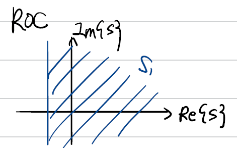
사실 주의해야할 점이 있습니다. f(t)는 t<0일 때 0이라는 조건이 있기 때문에 위와 같은 조건이 성립합니다.일반적으로 말하면, $-\infty$부터 $\infty$까지 $ |f(t) e^{-st}|$ 가 무한보다 작아야합니다.그리고 그렇게 만들 수 있는 s의 범위를 Region of Convergence(이하 ROC)라고 합니다.
Region of Convergence는 각 f(t)마다 모두 존재합니다. ROC의 정의를 따지자면 다음과 같습니다.
$\{s : Re(s) \geq \alpha | \alpha\text{ is the smallest real number for which F(s) and } Re(s)=\alpha\}$
예를 들면,
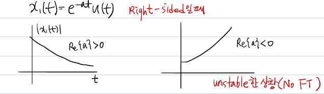
다음과 같이 $x(t) = e^{-at} u(t)$ 일 때, Laplace transform을 구해보면
$\int_{0}^{\infty} e^{-(s+a)t}dt = -\frac{1}{s+a} e^{-(s+a)t} \vert_{0}^{\infty} =-\frac{1}{s+a} (e^{-(s+a)\infty} - 1) = \frac{1}{s+a}$
여기서 전제는 $e^{-(s+a)\infty} = 0$입니다. 그래야만 Laplace transform이 존재할 수 있기 때문이죠.
따라서 $Re(s) > -Re(a)$ 임을 알 수 있습니다. 즉, 만약 $ -Re(a) = \alpha$라면 ROC는 ${s : Re(s) > \alpha}$ 입니다. (부등호에 등호 표시가 없는 것 주의! 만약 $ Re(s) = \alpha $일 경우 exponential이 상쇄되면서 간단하게 1이라고 했을 때도 무한으로 더하면 발산하기 때문입니다.)
4. Example
각 함수에 대한 Laplace transform은 직접 유도해볼 수도 있고, table을 찾아서 사용할 수도 있습니다.
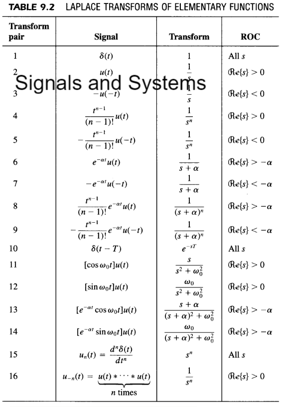
자주 Laplace transform을 까먹어서 저장해놓는 표입니다. (저작물에서 가져온 것이니 다른 곳으로 배포금지)
직접 유도해보면 기억이 더 잘 남으니 유도해보시는 걸 추천드립니다.
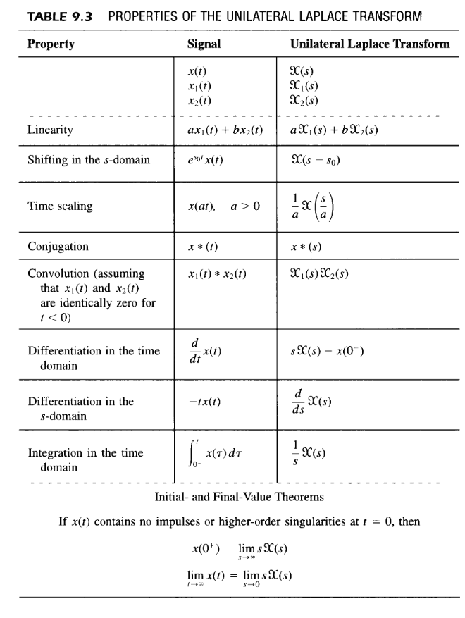
5. Properties
Linearity부터 해서 Final Value Theorem , Initial Value Theorem까지 다 다루려고 했으나 위에서 언급한 Signals & Systems에서 표로 잘 정리되어 있으므로 중요한 것들만 증명을 하려고 합니다.
참고로 Unilateral Laplace transform의 property임을 주의해야 합니다.
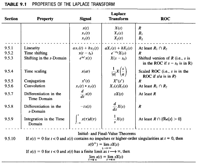
Laplace transform일 때와 property가 조금 다릅니다. (맨 아래에 Laplace transform의 properties를 올려놓겠습니다.)
# 위에 나와있는 성질에서 더 추가
$\text{ 1) Time delay (Time shifting)}$
$\mathcal{L}\{ x(t-\alpha)\} = e^{-\alpha} X(s)$
$\text{ 2) Integration in the s-domain}$
$\mathcal{L} \{\frac{x(t)}{t}\} = \int_{s}^{\infty} X(z) dz$
# Initial Value Theorem(IVT)와 Final Value Theorem(FVT) 증명
$ \mathcal{L} \{\frac{dx}{dt}\} = sX(s) - x(0) $ 에서 출발한다.
$ \int_{0}^{\infty} \frac{dx}{dt} e^{-st} dt = \int_{0}^{\infty} \frac{dx}{dt} \cdot 0 dt \text{ for } s \rightarrow \infty $
따라서
$ \lim_{s \rightarrow \infty} sX(s) - x(0) = 0 $ 이므로
$ \lim_{s \rightarrow \infty} sX(s) = x(0) \Rightarrow IVT $
비슷한 방식으로 FVT를 증명할 수 있습니다.
$\int_{0}^{\infty} \frac{dx}{dt} \cdot 1 dt = x(\infty) - x(0) \text{ for } s \rightarrow 0 $
$ x(\infty) - x(0) = \lim_{s \rightarrow 0} sX(s) - x(0)$
$ x(\infty) = \lim_{t \rightarrow \infty} x(t) = \lim_{s \rightarrow 0} sX(s) \Rightarrow FVT$
6. Inverse Laplace Transform
실제 문제를 풀 때 Laplace transform을 이용해 s domain에서의 output 결과를 알고나면 다시 time domain으로 변환을 해주어야 합니다. 그런데 Inverse Laplace transform의 식은 무척 어렵기 때문에 식으로 구하기 보다는 table을 보면서 변환하게 됩니다.
그래서 실제 문제에서 Inverse Laplace Transform을 사용하는 케이스는 2가지입니다.
1) 분수 꼴로 나오거나
2) exponential 함수 꼴로 나오거나
입니다.
분수 꼴로 나타나 있을 때는 각각을 부분분수로 분해한 다음에 각 분수를 원래 식으로 바꿔주면 됩니다.
예를 들면,
$\dot{y}(t) = -ay(t) \text{, initial condition : }y(0_{-}) = y_{0}$
$sY(s)-y(0_{-}) = -aY(s)$
$Y(s)=\frac{1}{s+a}y(0_{-})$
이 Y(s)는 분수 꼴이다.
따라서 inverse Laplace transform을 하면
$y(t) = e^{-at}{y_{0}}$
일반적인 Laplace transform이라면 ROC를 보고 inverse Laplace transform을 적용해야하지만
지금은 무조건 t<0일 때 함수값이 0이므로 결과는 하나로 정해집니다.
exponential 함수 꼴인 경우는 기본 식에 time delay가 있었던 경우입니다.
$ \mathcal{L} \{x(t-T)\} = e^{-sT} X(s) $
Bilateral Laplace transform의 properties
'연구 Research > 제어 Control' 카테고리의 다른 글
| [고등자동제어] System modeling (2) | 2020.12.03 |
|---|---|
| [고등자동제어] State space와 transfer function의 관계 (2) | 2020.11.19 |
| [고등자동제어] State space model (0) | 2020.11.18 |
| [고등자동제어] Z-transform (0) | 2020.11.17 |
| [고등자동제어] Introduction (2) | 2020.11.12 |